Discussion

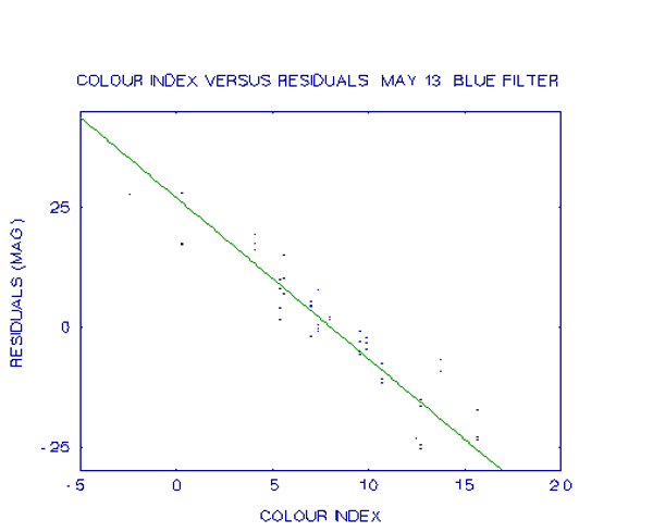
As more observations were obtained, the large residuals remained and considerable time was spent trying to identify their origin. Recordings and measurements were thoroughly checked and found to be correct. It was discovered that standard stars from different catalogues should not be mixed, but when the data was analysed separately for the two catalogues, it was found to make little difference to the residuals. It was not until, following a suggestion by P. Birch, that a plot be made of the residuals versus colour index, that a clue to the problem was found. This plot is shown below.

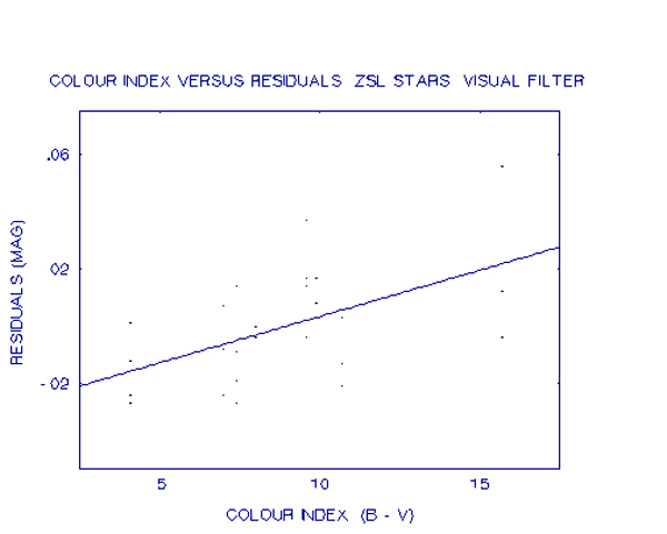
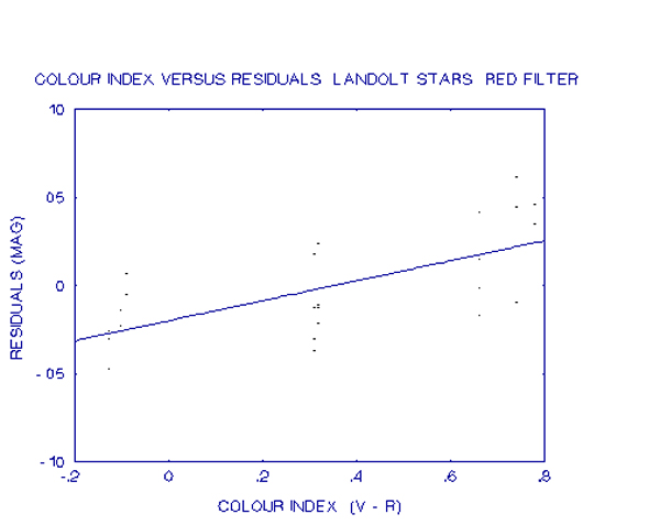
As can be seen, there is a strong correlation between colour index and the residuals. Similar plots were made for the visual and red filter observations but here the correlation is much weaker. These plots are shown in the next two graphs.

After much discussion it was realised that the problem lay with the PHEX program. Unlike I had originally understood, the PHEX program does not derive transformation coefficients. Rather, it has transformation coefficients for the photometer built in. Different photometer systems generally have only small differences between them so the transformation coefficients would be expected to be small. However, a CCD system has a very different spectral response to a photo-multiplier. In particular, as shown earlier, the response of the CCD system used at the Perth Observatory is dying away very rapidly across the bandwidth of the blue filter. This means that a red star will be recorded more intensely than a blue star of the same magnitude. The response of a photometer however is still rising across the blue filter bandwidth and so will record a blue star more intensely. The different spectral responses is the reason for the comparatively large blue transformation coefficient for the CCD, since it differs substantially from the system used by Johnson and Morgan when the UBV system was established.

The next table shows the transformation coefficients and zero points obtained with and without this star.

As can be seen from the tables, the inclusion of just one erroneous star can markedly affect the results. Without actually plotting the results, it is virtually impossible to deduce which star(s) is (are) causing the problem. While the use of computer-pointing of the telescope should minimise the risk of mis-identification of stars, there is still the possibility of variation in the sky conditions and extinction during the night which can cause problems for all-sky photometry. If the values are plotted on a graph, the erroneous stars should be readily identifiable. An example of this is shown in the next graph, which is a graph of the visual filter observations of January 11, 1993. Again on this night the pointing of the telescope was done manually using the finderscope and some stars were incorrectly identified. The graph itself is a plot of (V-v) - å(B-V) versus X, which is the method of finding the extinction coefficient from a number of standard stars with known transformation coefficients. The slope of the line of best fit will give the extinction coefficient. The transformation coefficient used is the ZSL coefficient derived on May 13.

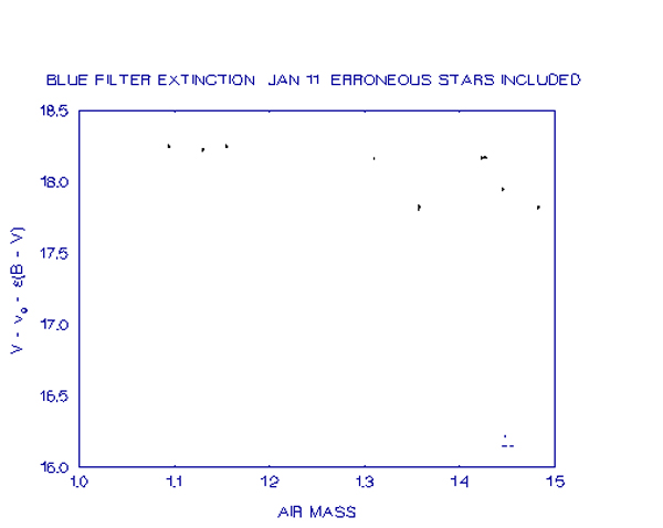
As can be seen from the graph, one star is immediately obvious as being deviant and this has distorted the extinction coefficient to a value of 1.94 magnitudes per air-mass. The deletion of this star from the graph reveals three further stars which have deviant values but were not noticeable on the scale of the first graph. With these stars included the extinction is still a very excessive 0.842 magnitudes per air-mass. This is shown in the next graph.

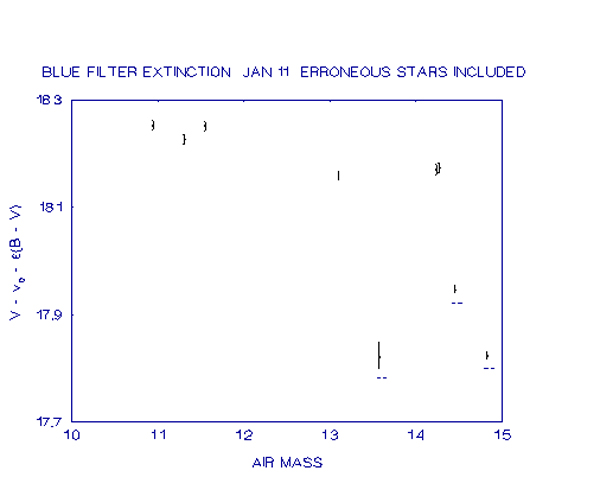
Once these other three erroneous stars are deleted, the extinction coefficient becomes a much more acceptable 0.264 magnitudes per air-mass. The same effects were seen in the blue filter observations. From this and the extinction examples referred to earlier it is evident that some provision for displaying the data graphically before calculating coefficients, to give the observer the opportunity to delete deviant observations, would be a very useful addition to a photometry program.

The biggest problem is the length of time required to obtain blue images. The observations have shown that for equal exposure times, the blue images are typically in the order of 10% of the intensity of visual images. This means that blue images require longer exposure times to acquire. As an example, 5 minute exposures on 13th magnitude stars still did not provide a peak signal of 100 ADUs above the sky background and it was necessary to use growth curves to determine the total count. For fainter objects very long exposures would be required which would severely reduce the number of observations possible per night. The graph below is a plot exposure times require to reach a total count of 2 x 104 ADUs for stars of various magnitudes. This count level was used as it was found to be about the lowest count that gave smooth growth curves.

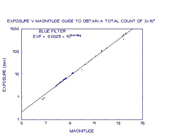
As can be seen from the graph, very long exposure times are required for faint stars. This means that the observer has to choose between long exposures, which means fewer observations and the possibility of telescope tracking errors, or weakly recorded images which require the use of a technique such as growth curves to derive the total count, which has the potential to reduce accuracy, as found in the project. Either that or to confine blue filter observations to the brighter objects. These problems would be much reduced if a CCD chip that has been coated to improve the blue sensitivity was acquired.

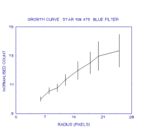
This conclusion has some support in a comment made several times by P. Birch from the Perth Observatory, in which he said that he felt it was not possible to perform photometry at the Perth Observatory to an accuracy of better than about 0.02 magnitudes for an individual observation of a star around 8th magnitude, due to its location. To improve upon this would require repeated observations. Being situated downwind from the city of Perth means that pollution from the city will pass over the Observatory so patches of smoke or haze could easily cause scatter in the observations, as evidenced in the previous section. A second problem with the location is its low altitude. A low altitude means a much greater amount of atmosphere for the star's light to pass through so distortions in the image due to turbulence in the atmosphere is much greater. An example of this is in the point at which the growth curves flatten out. My observations have shown that the growth curves do not flatten out until around 20-25 pixels radius, whereas Howell, observing with a 0.91 m telescope at Kitt Peak Observatory in Arizona, found the growth curves flattening out after about 12 pixels. This shows that the greater atmosphere at the lower altitudes of Perth has spread the star's light over a larger area of the CCD chip. The larger area means there is greater potential for errors to creep in unnoticed during the analysis.

These are factors which are unavoidable and must be accepted. For differential photometry where the object of interest and the comparison star(s) are usually very close to one another, the effect of haze or smoke patches would not be so great and could possibly be identified by an analysis of the residuals with respect to time, provided there are sufficient observations of each star. However, the scatter due to air-turbulence would remain and could well be greater than the scatter due to extinction fluctuations.

For all-sky photometry, where observations are made over a large area of sky and only a few observations are made of each object, it would be very difficult to identify sources of scatter and so it may be necessary to accept that this is the limit to which all-sky photometry may be undertaken with the present equipment at its current location.

The most obvious solution to this problem is to increase the exposure so that the star is recorded sufficiently strongly for a standard curve to be fitted. While this may be possible for standard stars which are relatively bright, it may not be possible for other objects which may lie near the limit of detectability, for example, a supernova. With exposure time increasing logarithmically with decreasing brightness, a very large increase in exposure time could be required, as discussed earlier, along with the disadvantages of a long exposure.

A possible solution in this situation is to examine the growth curves for other, brighter stars in the field to determine a standard curve for that image and then apply that curve to the object. For standard stars this is not usually possible because in most instances there are no other bright stars in the image. However, for other objects it would normally be expected that there would be other stars in the image.

It can be seen that the annulus size makes little difference until the size is below 25 pixels for the inner radius, where light from the star begins to be visible, thus raising the apparent level of the sky background and therefore lowering the star count. This means that the observer is free to choose the annulus size providing the inner radius is large enough to exclude the light from the star and the outer radius is not so large as to include other stars.

For non-isolated stars the situation is different. The next table lists the data gained for three stars on an image of supernova 1993K taken on April 15. Star 1 is a star near the nucleus of the galaxy, star 2 is the supernova, which is situated near one of the spiral arms, and star 3 is an isolated star near the edge of the field. Again the star aperture radius is 15 pixels.

As can be seen, the annulus size makes a considerable difference to the count. For the two stars within the image of the galaxy the total count varies widely, but in different ways. For the star near the nucleus the count decreases steadily as the size of the annulus increases. The most probable explanation for this is that near the nucleus the brightness of a galaxy generally increases steadily as the centre is approached. Therefore, as the annulus size is increased, the apparent brightness of the sky background will increase steadily, reducing the ADU count for the star. In the spiral arms however things are different as the brightness of the spiral arms can vary irregularly due to the presence of unresolved star clusters and bright and dark nebulae. Therefore the apparent brightness of the sky background can vary irregularly causing the star's ADU count to vary irregularly, as is seen for star 2. The changes need not be large since only a small change in the sky background count can have a large impact on a faint star.

The ADU count for star 3 does fluctuate, however the fluctuations are irregular and within the error bounds. Some of this fluctuation is possibly caused by imprecise flat-fielding since only one flat-field was used rather than the mean of several.

The consequence of this ADU count variation with annulus size is that the radii for the annulus must be chosen with care. In general, it should be kept as small as possible, to have the background within the annulus resemble the background at the star as close as possible. However, it should not be made so small that it includes some light from the star. In this regard, the skill and experience of the observer could play a significant role as each situation would need to be looked at individually.

Determining growth curves for some of the bright and more isolated stars on the image, and measuring the stars near the galaxy with small aperture radii where any errors due to sky background problems are lessened, would probably improve the accuracy. The growth curves could then be used to find the total count at larger radii. The alternative is to use the Point Spread Function method of photometry described in earlier.

An example of using growth curves is shown in the following graph, where an image of supernova SN1993K has been used. This was a visual filter image taken on May 13 by R. Martin. The size for the annulus used was the same as for the standard stars observed, namely, inner radius 40 pixels, outer radius 45 pixels.

As can be seen from the graph, the more isolated comparison stars show smooth growth curves except for one which was situated near a spiral arm of the galaxy. Here the annulus has apparently included part of the spiral arm, thereby increasing the sky background reading, whereas the star aperture has not. This means that as the star aperture has increased, a too higher value for the sky background has been subtracted, causing the growth curve to dip. Even so, at small radii, it matches the others closely, lending support to the earlier discussion.

EASYPLOT was used to fit the earlier equation to a mean curve and this resulted in a value for "e" of 1.762. This means that the total ADU count is 1.762 times the count with a 4 pixel radius.

Turning to the growth curve for the supernova, it is evident that it is very different. Being situated close to a spiral arm, the large annulus has included a region brighter than the background near the star. Since the star is quite faint, any deviations of this nature will have substantial effects. Indeed, in this case, as the star aperture increased, the count for the star went negative! Here is a situation where a combination of small radii for the annulus and the mean growth curve from the other stars would result in a much better determination of the total count.

This variation can come from two sources. In the lower atmosphere, the local weather can play a major role. The direction of the wind, humidity, proximity to rain, all effect the transparency of the atmosphere. In the upper atmosphere patches of volcanic dust can be a significant factor. For example, the general sky transparency has still not yet recovered to its level of the 1980s prior to major volcanic eruptions in the Philippines and South America. Some unusual sunsets were still being observed on occasions in 1992, indicating that clouds of volcanic ash were still in the atmosphere.

There were however some points which did not fit this line. The Landolt value for January 27 is lower than the value for May 13 and the ZSL value for April 28 is well below the other ZSL values. The Landolt value may well be unreliable since only five stars were used in its estimation, however the value for April 28 cannot be explained in this way. One possible explanation is that the extinction coefficient is not accurate due to the small air-mass range.

The B-V zero point also shows a steady decline, about 0.03 magnitudes per month.