These exposure times were chosen as these provided the greatest range of magnitudes. To make some allowance for the various zenith distances for the observations, an extinction correction was applied to the observations. While extinction is highly variable from night to night, applying a generic correction to the observations would remove much of the scatter that would have been otherwise present. The correction factors applied were:
visual filter 0.25
blue filter 0.32
Thus the correct counts were given by:
corrected count = raw count + 0.25 x air mass (X) (visual filter)
corrected count = raw count + 0.32 x air mass (X) (blue filter)
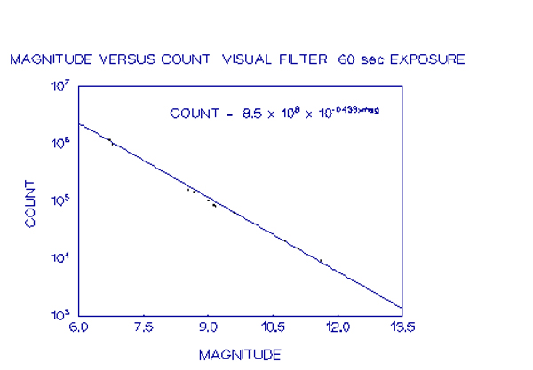
These factors were chosen because they were around what was expected from previous photometric observations by other observers. As was subsequently found, these values were a little on the low side, however they were close enough for the purposes of this analysis. The results are shown below.
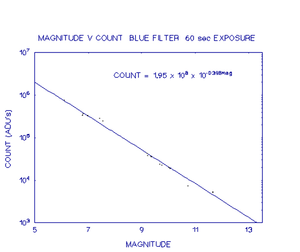
As can be seen from the graphs, the points all lie very close to a straight line fit, showing that over the range of counts recorded, the CCD is linear. Most of the scatter is likely to be from two sources - the use of a fixed extinction coefficient for several different nights and no application of transformation coefficients to account for differing colour indices.
In view of this result, it was felt that there would be no additional errors generated by normalising the exposures to a single value. The equations were calculated using the curve-fitting routine from the EASYPLOT package to fit an exponential curve to the data.
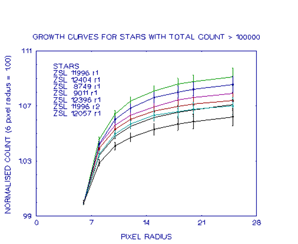
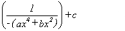
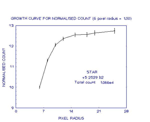
In this graph, a number of stars with high counts (< 1 x 10^5) are shown. It will be noticed that each of these curves has the same basic shape, differing only by a constant. This variation comes largely from using star profiles from different images rather than from the same image as Howell was able to do. These curves can be represented by the quartic equation:
The EASYPLOT routine was used to fit a mean curve to this set of plots and this gave the following values for the coefficients:
a = 1.35 x 10^-3
b = 0.3267
c = 1.081
The graphs below show stars which had progressively lower total counts
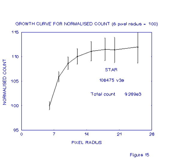
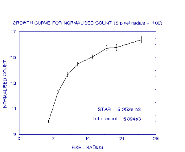
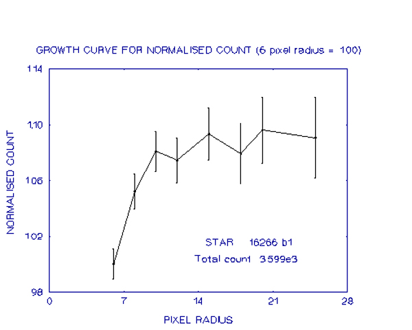
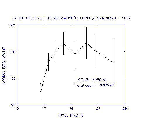
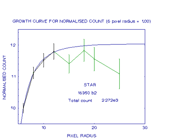
An examination of these graphs shows how, as the total count becomes less, the growth curves become more irregular, due to the sky background contamination, as discussed earlier. Despite this irregularity however, the curves are still well-defined at small pixel radii and so it is possible to fit the above equation to the measurements of these small pixel radii and from there find the total count more precisely. An example of where this has been done is for the last of the graphs.
The derived curve has coefficents of:
a = 9.321 x 10^-4
b = 9.955 x 10^-2
c = 1.208
These are in broad agreement with those derived earlier for the more intensely recorded stars. Again the main contribution to the variation would come from the stars being on different images. The value of 1.208 for "c" indicates that the limiting value for the ADU count at large aperture radii is 1.208 times the value at 6 pixels, which yields a total ADU count of 2.934 x 10^3 The curve generated by the equation using these coefficients is shown in the graph below, superimposed on the actual growth curve. As can be seen, the fit is very good except at large radii.
A problem with this process is that there could be a variety of curves that will match the growth curve of the star. With most images there would be a number of stars on the image and so several growth curves could be generated and a mean equation used, as recommended by Howell[16]. However, with many standard stars there are no other stars in the image, so this cannot be done. This means that there is the possibility of an error in the derived count that is difficult to estimate. Despite this, the results should still be more accurate than if no growth curve was used. Also, when deriving the coefficients using EASYPLOT, it was found that a shift of 0.01 in the value of "c" would prevent an accurate fit to the data points.
In order to obtain some idea of how much any error could be, only standard stars which produced a total count of greater than 2 x 10^4 ADU were used to determine the extinction and transformation coefficients and then these coefficients were used to calculate the magnitudes of standard stars with lower counts. The residuals could then be examined to check if deviations were noticeably greater than for those with higher counts. The results of this are presented in the following table.
|
|
|
|
|
|
|
|
|
|
|
|
|
|
|
|
|
|
|
|
|
|
|
|
|
|
|
|
|
|
|
|
|
|
|
|
|
|
|
|
|
|
|
|
|
|
|
|
|
|
|
|
|
|
|
An examination of the table shows that most of the residuals are of similar size to those of other stars shown in the appendices. The observations which show large residuals are discussed in a later section.
|
|
|
|
|
|
|
|
|
|
|
|
|
|
|
|
|
|
|
|
|
|
|
|
|
|
|
|
|
|
|
|
|
|
|
Several different methods were used to calculate the extinction. On January 27 observations were made of the A-type star ZSL 9232 over a variety of air-masses. The extinction coefficients were then calculated using the method outlined on page 19. The data was plotted using the EASYPLOT package and a least-squares fit was used to find the coefficients.
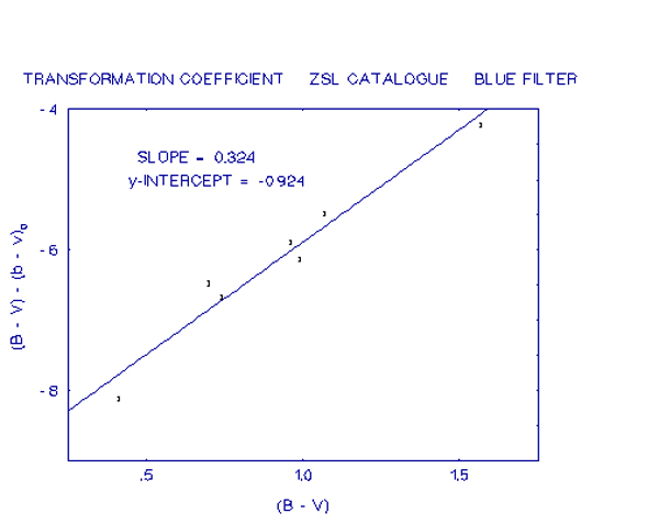
The next table lists the data while the following graph is an example of the data plotted in graphical form, in this case the blue filter observations. Although no (V-R) data is included in the ZSL catalogue it was still possible to calculate the (V-R) coefficient since only one star was used and the inclusion of such data would only add a constant to each point on the graph, not changing the slope of the line of best fit.
|
|
|
|
|
|
|
|
|
|
|
|
|
|
|
|
|
|
|
|
|
|
|
|
|
|
|
|
|
|
|
|
|
|
|
|
*The air-mass value given is the mean of the three observations. The actual values were used in the calculations.
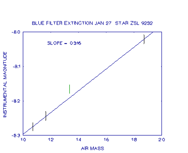
Looking at the above graph, it can be seen that the third observation is some distance above the line of best fit. This indicates it is fainter than expected. Observations with each filter at this time show this effect. This is an illustration of the caution given earlier about using a computer only to find the extinction coefficients rather than actually plotting the values. Here it is likely that a thin patch of haze was passing the star when the observations were being made. Accordingly, these points were ignored when finding the extinction coefficients.
The coefficients for May 13 were calculated by hand using three stars from the Landolt catalogue which were observed several times each. It had been intended to also use four stars from the ZSL catalogue to compare the effects of using different catalogues. However, subsequent analysis showed that one set of observations had to be discarded as a result of the CCD warming up after running out of liquid nitrogen. This left insufficient observations to make meaningful calculations using the ZSL stars.
For each of the three Landolt stars, the observations were plotted on a graph using EASYPLOT and then the line of best fit found, the slope of which gave the extinction coefficient for that star. The three coefficients were then averaged to give the coefficient for the night. This process was followed for all three colours. The next table lists the results obtained, along with the means.
|
|
|
|
|
|
|
|
|
|
|
|
|
|
|
|
|
|
|
|
|
|
|
|
|
|
|
|
|
|
|
|
|
|
|
|
The extinction coefficients for April 27 were calculated by using all the stars observed and the transformation coefficients calculated from the May 13 observations. On this occasion the coefficients were calculated using the EXTINC routine from the photometry package by Kaitchuck and Henden.
The extinction coefficients for January 11 were also calculated using the transformation coefficients derived on May 13, but in this case, the data were calculated by hand and the results plotted using EASYPLOT. The reason for this will be discussed in the next section.


Here the subscripts 1 and 2 refer to the two stars. All other coefficients are the same as in the earlier equations. When the above plots are made the result is a straight line with slope K".
The following tables contain the data for each filter and an example of the resulting graph follows.
|
|
|
|
|
|
|
|
|
|
|
|
|
|
|
|
|
|
|
|
|
|
|
|
|
|
|
|
|
|
|
|
|
|
|
|
|
|
|
|
|
|
|
|
|
|
|
|
|
|
|
|
|
|
|
|
|
|
|
|
|
|
|
|
|
|
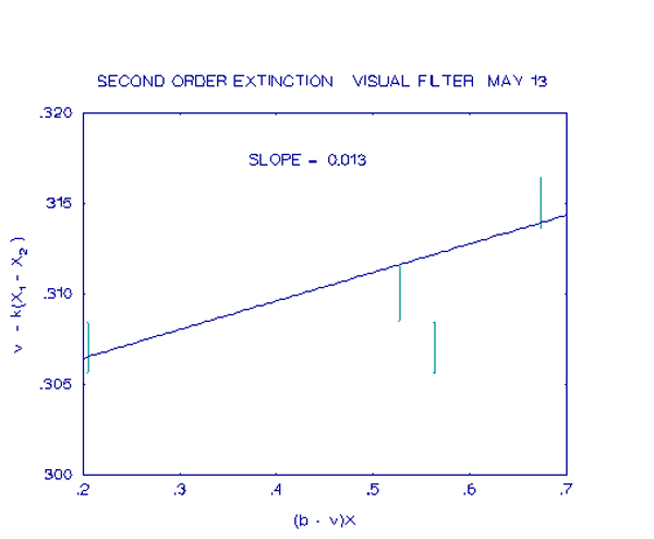
In the following table, the first column for each star contains the raw instrumental magnitude (i.e. uncorrected for extinction), column 2 lists the air-mass, and column 3 lists the raw instrumental b-v colour index. The fourth columns are the product of the second and third columns. The final two columns in the table are the difference in the raw instrumental magnitudes minus the difference in air-mass times the extinction coefficient and the difference between the raw instrumental colour index times air-mass. These values were plotted using EASYPLOT and a least-squares fit was used to fit a straight line to the data, the slope of which gives the second-order extinction coefficient K", which is given below each table. The next two tables contain the same type of information except that colour indices are used rather than magnitudes so therefore only three columns are required for each star.
|
|
|
|
|
|
|
|
|
|
|
|
|
|
|
|
|
|
|
|
|
|
|
|
|
|
|
|
|
|
|
|
|
|
|
|
|
|
|
|
|
|
|
|
|
|
|
|
|
|
|
|
|
|
|
|
|
|
|
|
|
|
|
|
|
|
|
|
|
|
|
|
|
|
|
|
|
|
|
|
|
|
|
|
|
|
|
|
|
|
|
|
|
|
|
|
|
|
|
|
|
|
|
|
|
|
|
|
The data for each filter shows quite some scatter. Much of this is due to using the difference between star magnitudes which will emphasise small deviations. In view of the small number of observations no great accuracy can be claimed for these results, although it is reassuring to notice that the results are very similar to those derived using the photomultiplier.
|
|
|
|
|
|
|
|
|
|
|
|
|
|
|
|
|
|
|
|
|
|
|
|
|
|
|
|
|
|
|
|
|
|
|
|
|
|
|
|
|
|
|
|
|
|
|
|
|
|
|
|
|
|
|
|
*The air-mass value given is the mean of the two colours. The actual values were used in the calculations.
In the above table, the first column is the catalogue designation of the star, the second column is the air-mass, the next two columns are the instrumental magnitudes and colour indices corrected for extinction and the final columns list the differences between the catalogue and instrumental values. It is the data in these final two columns which is plotted against the catalogue colour index to derive the relevant colour index. Table 10 is the same except that two extra columns have been added to include the V-R colour index.
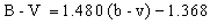
Using the graph below as an example, the earlier equation shows that the slope is
(1 - 1/ě) and the zero point is îbv/ě . From the graph the slope is 0.324.
Therefore 1 - 1/ě = 0.324
so ě = 1.479
The y-intercept is -0.924
therefore îbv/ě = -0.924
so îbv = 1.367
The slight difference between these values and those given in the earlier tables, is
caused by round-off error within the COEFF routine which was used to derive the
values given in the tables.
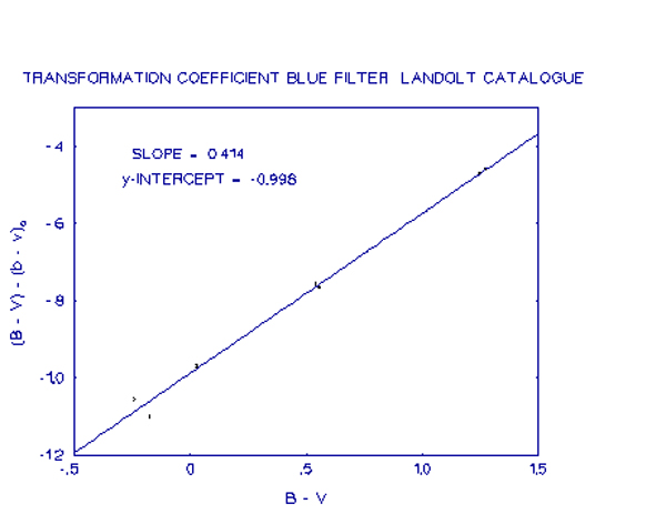
The same process was followed in calculating the transformation coefficients for the Landolt stars. The following tables show the data while the next graph is an example of the data plotted graphically. Then 2 tables list the trans-formation coefficients and the zero points calculated for each night.
|
|
|
|
|
|
|
|
|
|
|
|
|
|
|
|
|
|
|
|
|
|
|
|
|
|
|
|
|
|
|
|
|
|
|
|
|
|
|
|
|
|
|
|
|
|
|
|
|
|
|
|
|
|
|
|
|
|
|
|
|
|
|
|
|
|
|
|
|
|
|
|
|
|
|
|
|
|
|
|
|
*The air-mass value given is the mean of the three colours. The actual values were used in the calculations.
|
|
|
|
|
|
|
|
|
|
|
|
|
|
|
|
|
|
|
|
The values contained in Tables 11 and 12 were calculated using the COEFF routine from the photometry package by Kaitchuck and Henden.
|
|
|
|
|
|
|
|
|
|
|
|
|
|
|
|
|
|
|
|
|
|
|
|
|
|
|
|
|
|
|
|
|
|
|
|
|
|
|
|
|
|
|
|
|
|
|
|
The formulae used were:


The zero points given in the above equations were for observations made on May 13. For the other nights the appropriate zero point was substituted. A summary of the results is shown in the table below.
|
|
|
|
|
|
|
|
|
|
|
|
|
|
|
|
|
|
|
|
|
|
|
|
|
|
|
|
|
|
|
|
|
|
|
|
|
|
|
|
|
|
|
|
|
|
|
|
|
|
|
|
|
|
|
|
|
|
|
|
|
|
|
|
|
|
|
|
|
|
|
|
|
|
|
|
|
|
|
|
|
|
|
|
|
|
|
|
|
|
|
|
|
|
|
|
On February 3 the extinction was calculated using five observations of the star ZSL 9232, while on March 15, eight observations of the star ZSL 10553 were used. The second order extinction was calculated using one pair of stars on March 15. The table below lists the results obtained.
|
|
Range |
|
|
Extinction |
|
|
|
|
|
|
|
|
|
|
|
|
|
|
|
|
|
|
|
|
|
|
|
|
|
|
|
|
|
|
|
|
|
|
|
|
|
|
|
|
|
|
|
|
|
|
|
|
|
|
|
|
|
Magnitudes for all the stars observed were then calculated using the equations above with the appropriate coefficients, and the results are shown in Appendix D. A summary of the results is shown in the table below.
|
|
|
|
|
|
|
|
|
|
|
|
|
|
|
|
|
|
|
|
|
|
|
|
|
|
|
|
|
|
|
|
|
|
|
|
|
|
|
|
|
|
|
|
|
|
|
|
The CCD B-V zero points are negative while the photomultiplier B-V zero points are positive. This shows that the photomultiplier is more sensitive in blue than in visual, while the CCD is the reverse. A comparison of Tables 13 and 15 shows that the accuracy of the two systems is very similar in both the extreme residuals for each night and in the standard deviations. This point is discussed further in a later section.
p>|
|
|
|
|
|
|
|
|
|
|
|
|
|
|
|
|
|
|
|
|
|
|
|
|
|
|
|
The magnitudes of the comparison stars and the supernova were calculated for May 13 using the Landolt transformation coefficients. The results are shown in the table below. The Landolt transformation coefficients were used so as to give red filter values.
|
|
|
|
|
|
|
|
|
|
|
|
|
|
|
|
|
|
|
|
|
|
|
|
For reasons which are discussed earlier, growth curves were used to derive the total count for each star, including the supernova. The mean growth curve for the comparison stars was used. Also for reasons given in section 6.5, an annulus of radii 27 and 30 pixels was used for sky background estimation. Smaller radii would have been preferred, however some of the images, particularly from May 13, were badly trailed due to telescope tracking problems.