METHODS

On each night, stars were selected from the Landolt and/or ZSL catalogues with the aim of covering a wide range of spectral types and zenith distances. A range of magnitudes was also chosen in order to check the linearity of the CCD for both high and low counts and to examine the growth-curve behaviour at low counts. It was originally intended to observe the same stars on many nights, however this was only partially achieved.

On the first three nights with the CCD, pointing of the telescope was done manually using the finderscope mounted on the side of the main telescope due to problems with the computer aiming program and imprecise star positions. This was found to be unsatisfactory due to problems of unambiguously identifying the star and of being very slow. Therefore, on the final two nights, positioning was done by computer, which was much more effective.

The photometric observations were made in a set sequence of V star V sky B sky B star, and the data recorded on floppy disk. Sky readings were made by shifting the telescope slightly so that it was aimed at a blank region of sky. These results were then fed into the PHEX program to obtain magnitudes and extinction coefficients. The results were also run through the package by Kaitchuck and Henden to provide comparisons with the PHEX results and the CCD results.

In making the CCD observations the observing run was commenced by taking a number of bias images (usually 2-4). On May 13, when the observing session lasted most of the night, further bias images were taken during the night to ensure there was no change.

Following the bias images, flat field images of the twilight sky were obtained. Usually three images of the twilight sky through each filter were obtained. Exposures varied depending on the filter being used and the brightness of the sky but were usually between one and three minutes and were aimed to give an ADU count per pixel of at least 5000 following bias subtraction. Most of the bias and flat-field images were taken by R. Martin and A. Williams as part of their supernova search program which was running concurrently.

Once the flat-fields were taken, observations were made, initially using blue and visual filters, and later also using the red filter. Exposures varied according to the brightness of the star and the filter being used and varied between 20 seconds and 420 seconds. On May 13 some exposures were deliberately kept short to mimic observations of faint objects. Occasionally some images had to be retaken when the exposure was found to be either too long and the image saturated or too short, so the object was very weakly recorded.

Following bias subtraction the flat-field images for each filter were added together and divided by the total number of images for that filter. This process provided a mean flat-field for each filter. Again the reason for this was to minimise the effects of random noise.

The mean pixel count on the averaged flat-field images was then found using the "MN" command. This command finds the mean pixel count value and stores that value in the computer's memory.

The first step in analysing the star images was to subtract the bias, then the images were flat-fielded using the DIVIDE........FLAT command. With this command, each pixel count on the flat-field image is divided by the mean value stored in the memory, thus setting each value as a ratio of the mean. The star image is then divided by these ratios on a pixel-pixel basis, i.e. Pixel (i,j)star is divided by pixel (i,j)flat / flat mean. This process largely compensates for any variations in pixel sensitivity.

Once the image has been flattened the SKY command was used to find the mean sky background. This routine calculates the sky background by using the assumption that the mode of the pixel counts is the sky background level. A histogram is built up of pixel intensities and the value for where the peak occurs is used as the sky background value. This method means that star images have minimal effect on the calculation. The error in the measurement is derived by fitting a gaussian to the histogram peak and finding the standard deviation. The values are printed on the screen and stored in memory.

The next step was to use the MARKSTAR routine to identify to the computer the pixel location of the star to be measured. This is done interactively by placing a cursor over the star's image and finding the location of the peak value. Exact placement is not required as the routine can locate the exact point of the peak value providing the cursor is within the image of the star. Since the program also points out the intensity reading for the pixel upon which the cursor is located, this routine was used to find the peak count for the star image.

Once the star(s) of interest had been marked, the APERSTAR routine was used to find the total integrated count for each star. This routine uses a circular aperture with a radius specified by the user, to define the region covered by the star. The intensity of all the pixels within the aperture is summed to give the total count.

The routine also uses an annulus entered on the same pixel as the star aperture for determining the sky background. Here the intensities of the pixels within the annulus are summed and the sum is divided by the number of pixels to find the mean.

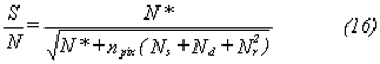
To find the total count within the aperture attributable to the star alone, the mean times the number of pixels within the aperture is subtracted from the total count. The result is printed on the screen in the form of position of the star on the image, the total count and the error. The error is calculated by using what Howell calls "the CCD equation",

Images are read into the package and stored in special memory allocations called buffers. Subsequent analysis is done using these buffers. The most frequently used routines in this project were the arithmetic routines for finding the mean of several images and for flat-fielding; the TV routine for displaying images; the MARKSTAR routine to identify to the computer objects of interest in the image; and the APERSTAR routine to perform aperture photometry on the objects selected using the MARKSTAR routine. It is the APERSTAR routine that calculates the ADU count for the object under study.

For this system, the read noise is 30 and the dark current when the system is at operating temperature is negligible.

In order to determine growth curves, the software aperture was varied between a radius of 6 pixels and a radius of 25 pixels. A variety of radii for the annulus were examined but it was found that for isolated stars the radii made little difference to the count or the error, providing the inner radius was greater than 30 pixels. As a result, radii of 40 and 45 pixels for the inner and outer edges were chosen. The resulting counts were then normalised to a 300 second exposure and the results were entered into the photometry packages described earlier to derive the magnitudes and coefficients.

Using observations of standard stars, the extinction coefficients and zero points are derived by one of the methods described earlier. Deviations from the catalogue magnitudes are calculated and stars which have a residual of more than two standard deviations are excluded from the analysis. The coefficients are then used to calculate the magnitudes of other objects and the results are printed out in a list.