In absolute photometry, the object under study is observed without reference to a particular comparison star and the ADU count is analysed to obtain the object's actual brightness. This is a much more involved process and will be discussed in more detail later.
The output amplifier converts the charge into a voltage which is converted into a numerical value by an analogue to digital converter.
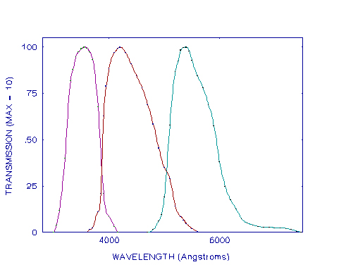
A set of ten bright stars were used to define the system and then a number of other stars were chosen to serve as secondary standards. From these secondary stars catalogues of photometric standard stars have been developed (e.g. Landolt). With the advent of red-sensitive detectors, this system was extended by Kron and Cousins to include R(ed) and I(nfrared), and is now commonly known as the Johnson-Kron-Cousins classification or sometimes just the Johnson-Cousins classification. Thus, by using the appropriate filters and observing the standard stars, observers can deduce the correction factors required to account for the systematic error induced by differing equipment sensitivities. These correction factors are known as transformation coefficients since they are used to transform the observations from the instrumental system to the standard system. They are calculated by comparing the catalogue and observed magnitudes for stars of differing colours. A more detailed discussion of this calculation process is contained in a later section.
Photometric observations and standard star lists are usually not published as a set of magnitudes for each colour but as a magnitude for one colour (usually visual) and then as colour indices for the other colours. The colour index is the difference between the magnitude of two (usually adjacent) colours with the longer wavelength colour being subtracted from the shorter, e.g. blue-visual (B-V), visual-red (V-R).
There are several other photometry systems for various photometric programs but the Johnson-Cousins system is most widely used and was used for this project.
Having secured images through the appropriate filters, bias-subtracted and flat-fielded them, it is necessary to calculate the ADU count for the object under study.
This image spreading means that it is necessary to sum the count from a number of pixels to find the total count from the star. There are two methods for doing this.
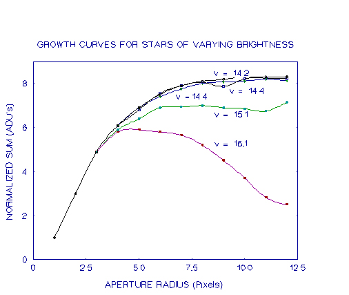
To overcome this problem, Howell recommends constructing "growth curves" for a number of bright stars to show how the ADU count increases as the aperture radius increases. Examples of this are shown in figure 3. This growth curve is a graph of the ADU count versus the pixel radius. For ease of plotting the ADU count is normalised to equal 1 at some small radius. Initially the curve increases very quickly but as the pixel radius increases further the curve flattens out until when most of the star's light is within the radius, there is little increase in ADU count with increasing radius. This point corresponds to the total ADU count for the star. Faint, weakly recorded stars do not show this smooth curve, is shown in the figure below. This is because as the star aperture radius is increased more pixels which are dominated by the sky background are included. Any form of error in the sky background subtraction will cause a faint star to deviate from a smooth growth curve. In the case of the figure below, the sky background has been slightly over-estimated, causing the curve to drop. The error need only be small, and as Howell points out, even truncation errors during processing can have an enormous effect on faint stars. However, a "standard" growth curve may be derived from other brighter stars and then fitted to the faint source using the values at small radii where sky-background contamination is not such a problem. This procedure is very likely to be necessary in the case of supernovae, where the star may be very faint and the background may be non-uniform.
Since most amateur photometry using this method, it is importand that the radius of the aperture be given careful consideration.
The usual method of doing this is to place a synthetic annulus larger than the object's image, concentric with the object. This annulus should be large enough to contain a large number of pixels and yet small enough to avoid contamination by other objects. An investigation was conducted into the optimum size of the annulus and the results are presented in section 6.5. The count within the annulus is averaged over the number of pixels and this value is used as the sky background per pixel. This value is then subtracted from the pixels within the aperture.
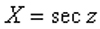
The first step in calculating the extinction coefficient is to calculate the air-mass through which the object's light is passing. For zenith distances of less than 60° the air-mass is given by:
If the zenith distance is greater than 60°, the above approximation breaks down and the following formula should be used :

Kaitchuck and Henden point out that because the above data are for only one location and are for average sky conditions from around the turn of the century, the air-mass calculation is only accurate to about 0.1%. This however is more than sufficient. The second step is to actually calculate how much the object's light is dimmed by this air-mass. There are several methods of doing this, depending on the type of observing program being undertaken.
If differential photometry is being performed then the observations of the comparison star may be used providing they span a range of at least 0.7 air-masses. If this is the case it is simply a matter of plotting the instrumental magnitude against X. This will give a graph of how the brightness varies with changing air-mass. The slope of the line of best fit will give the extinction coefficient.
In the case where objects are scattered around the sky and only a few observations of each object are obtained, there are two other methods available depending on whether or not the transformation coefficients are known.
Method 1 : Unknown transformation coefficients In this method, standard stars of spectral type A are observed for a range of air masses, and then the difference between the instrumental and catalogue magnitudes is plotted against air-mass. The slope of the line of best fit will give the extinction coefficient.
The actual equation for this using a visual filter is:
V - v = -Kv'(X) + ĺ(B-V) + îv
In this equation,
V is the visual catalogue magnitude;
v is the instrumental visual magnitude;
K'v is the first-order visual extinction coefficient;
X is the air-mass;
ĺ is the visual filter transformation coefficient;
(B-V) is the catalogue colour index of the star;
îv is the visual filter zero point.
(Throughout this paper capital letters refer to catalogue values and lower case letters refer to instrumental values. A subscript 'o' indicates instrumental values corrected for extinction.)
For an A-type star (B-V) is small and ĺ is also small so the equation may be approximated by:Method 2 : Known Transformation Coefficients When the transformation coefficients are known, any standard stars can be used to calculate the extinction coefficients. A minimum of five standard stars should be used at a wide range of air-masses. (Da Costa suggests 15-20 would be a more suitable number, while Massey et al report observing 5-7 standard stars, 7 to 10 times per night per filter). When the difference between the catalogue and instrumental magnitudes, minus the transformation coefficient times the colour index is plotted against the air-mass, the slope of the line of best fit will be the extinction coefficient.
The equations for this are:
V - v - ĺ(B-V) = -K'vX + îv
(B-V) - ě(b-v) = -ě K'bv X + îbv
(V-R) - ř(v-r) = -ř K'vr X + îvr
where ě and ř are the (B-V) and (V-R) transformation coefficients respectively, and îbv and îvr are the b-v and v-r zero points respectively. The first-order extinction coefficient is highly variable and needs to be determined each night.
The method used to determine the second-order extinction coefficient is to observe a pair of stars with as large a difference in colour index as possible over a range of air-masses. The pair of stars should be as close to each other as possible. A plot of the difference in colour index against the difference in colour index times the air-mass is then made and the slope of the line of best fit will be the extinction coefficient.
In mathematical terms:
Äv = K"v Ä(b-v) X + Ä vo
whereÄv is the difference in raw instrumental magnitudes;
Ävo is the difference in instrumental magnitudes corrected for extinction;
K"v is the visual second-order extinction coefficient;
Ä(b-v) is the difference in the raw instrumental colour index;
X is the air-mass.
Therefore plot ÄV versus Ä(b-v)X.
Similarly for the other filters :
Ä(b-v) = K"bv Ä(b-v)X + Ä(b-v)o
and plot Ä(b-v) versus Ä(b-v)X;
Ä(v-r) = K"vr Ä(v-r)X + Ä(V-r)o
and plot Ä(v-r) versus Ä(v-r)X.
Despite how carefully manufactured, all CCD chips and filter systems have slightly different responses. Also, the UBVRI system was developed using photomultipliers which have a different spectral response compared with CCDs. This means that a correction factor is required to convert the observations to the particular standard system that the observer is working with. This correction factor is dependent upon the colour index of the object and the correction factor is the product of a constant and relevant colour index. The constant reflects the sensitivity of the system in a particular colour in relation to the sensitivity of the equipment used to establish the standard system, and is known as the transformation coefficient.
The method for determining the transformation coefficients is to observe a group of standard stars as close to the zenith as possible. This is to minimise the effects of extinction. The stars should have a wide range of colour indices and Kaitchuck and Henden recommend that 10-20 stars be used. They suggest that half a night should be set aside for determining the coefficients as the extinction coefficients need to be accurately determined as well.
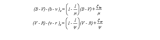
Once the instrumental magnitudes have been determined and corrected for extinction, a plot of the difference between the catalogue and instrumental magnitudes versus the colour index is required. The slope of the line of best fit will give the transformation coefficient. If colour indices are being used rather than actual magnitudes, the transformation coefficients will be equal to 1/(1 - slope). Hence, the equations are:
The transformation coefficients will vary slowly over time and so should be checked periodically. Kaitchuck and Henden suggest at the beginning and ending of an observing run.
For example, using the first of the two equations above, a plot of (B-V) - (b-v) against (B-V) will result in a straight line with slope (1 - 1/ě) and y-intercept îbv/ě , where ě is the transformation coefficient. Multiplying the y-intercept by the transformation coefficient will give the zero point.
Some researchers (e.g. Massey et al, Walker) have found that the zero point stays very stable during the course of an observing run, while others such as Kaitchuck and Henden think differently and feel that it should be calculated each night. Since the zero point is a reflection of the sensitivity of the system, a large change would indicate either an error in the analysis, perhaps caused by an incorrect star, or a possible problem with the system. In this way a calculation of the zero point can provide some indication of the accuracy of the data. Small variations in the zero point can arise from variations in sky transparency.
Routines for calculating the above coefficients are usually included in photometry packages for computers (e.g. Astronomical Photometry for the IBM PC).