UNIT 1
ONE-DIMENSIONAL MOTION GRAPHING AND MATHEMATICAL MODELING
Objectives
- To learn about three ways that a physicist can describe motion along a straight line – words, graphs, and mathematical modeling.
- To acquire an intuitive understanding of position, velocity, and acceleration for one-dimensional motion.
- To recognize how graphs can be used to describe changes in position, velocity and acceleration of an object moving along a straight line.
- To be able to use mathematical definitions of average velocity and average acceleration in one dimension.
- To check the validity of some of the standard kinematics equations used to describe the motion of objects undergoing constant acceleration.
- To be able to use kinematics equations to describe the motion of objects moving with constant acceleration.
Equipment list:
Masking tape
4 Stopwatches
1 Bowling Ball
Excel spreadsheet
1.1 Below are a series of snapshots of three different bowling balls at times t1, t2, t3, t4, and t5. The times are equally spaced. Suppose each of the time intervals is 0.5s.
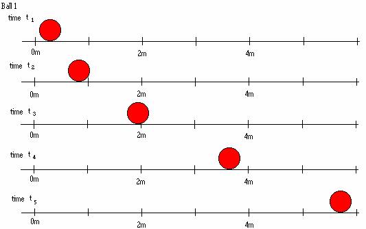
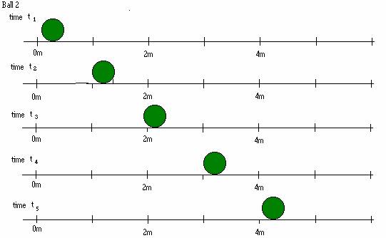
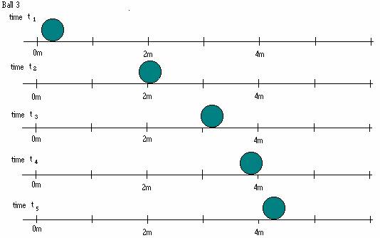
a. Determine if each bowling ball is speeding up, slowing down, or moving at constant speed. Explain your reasoning.
b. In the first time interval, compare the distances covered by each bowling ball. How does the distance covered in that time interval give you information about the speed of the bowling ball? Explain.
1.2 Obtain a bowling ball. With a piece of masking tape, mark off a starting point, and distances of 2m, 4m, 6m, and 8m from the starting point.
a. Predict what will happen, if you release the bowling ball at the starting point. Will it move at constant speed, speed up or slow down? If you record the time it reaches the 2m, 4m, 6m, and 8m marks, will the time intervals between adjacent marks increase, decrease or remain the same? Explain.
b. Perform the experiment. Release the bowling ball at the starting point. Use stopwatches, starting them at the time the ball is released, and recording the time the ball crosses the 2m, 4m, 6m, and 8m marks. Record the positions and times in an Excel spreadsheet.
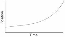
c. If you were to plot the position on the vertical axis and the time on the horizontal axis, what would the plot look like? (This is a prediction.)
d. In Excel, use Graph to plot the position on the vertical axis and the time on the horizontal axis. Explain why it looks the way it does. How does it compare to your prediction?
e. What would a graph of speed vs. time look like?
Discuss with an instructor.
Equipment list:
Motion detector
LabPro computer interface
LoggerPro software
2.1 An ultrasonic motion detector is a device that can be used to record an object’s motion as a function of time. It sends out a series of sound pulses (too high frequency to hear). These pulses reflect from objects in the vicinity and the reflected pulses return to the sensor. The computer can record the time it takes the reflected pulses to return to the computer, and using the speed of sound, calculate the position of the object.
When using a motion
sensor:
1. Do not get closer than
0.5 meters from the sensor because it cannot record reflected pulses that come
back too soon after they are sent.
2. The
ultrasonic waves spread out in a cone of about 15° as they travel. They will “see” the closest object. Be sure there is a clear path between the
object whose motion you want to track and the motion sensor.
3. The
motion sensor is very sensitive and will detect slight motions. You can try to glide smoothly along the
floor, but don’t be surprised to see small bumps in position graphs and even
larger bumps later in velocity and acceleration graphs.
4. Some objects like bulky sweaters are good sound absorbers and may not be “seen” very well by a motion sensor. You may want to hold a book in front of you if you have loose clothing on.
a. Predict and sketch position vs. time (time on the horizontal axis, position on the vertical axis) graphs for the following situations:
· standing still
· starting near the detector, walking at a fast steady walking speed away from the detector
· standing about 3m away from the detector, walking at a slow steady walking speed towards the detector, stopping briefly, walking at a fast steady walking speed away from the detector
· walking at a slow steady walking speed away from the detector, then walking at a fast steady walking speed further away from the detector
· walking away from the detector slowly, stopping for a while, walking faster away from the detector
b. At your table you have Motion Detector, a LabPro computer interface and the manuals that accompany that equipment. Connect the white (USB) cable to the computer and the other end to LabPro computer interface (See the Vernier LabPro User’s Guide or ask your instructor, if you have questions.) Connect the power cord to the AC adapter port on the LabPro computer interface and plug it in. Connect the gray British Telecom end of the cable into DIG/SONIC2 on the LabPro interface. Set the motion detector where you have an aisle in front of the detector about 5m long and 1.5m wide. Click on this link to the file Position, go to Setup, choose Data collection, under Sampling set experiment to about 3 sec. (You can change this. You will probably want it between 2 to 6 seconds, depending on what you are doing.) and set the samples per second to about 40. Click OK.
Perform the motions described in part a. in front of the motion detector while taking data.
c. Discuss with your partners the difference in your motion that produces differently sloped parts of the graph. Discuss moving forward and backward and how it affects the graph.
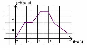
2.2 Consider the following graph.
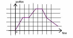
a. Describe in words how you would move
in front of the motion detector in order to
create the graph.
b. Walk in front of the motion detector and try to create the graph.
2.3 Consider the following diagram.
(from Workshop Physics (Electronic Version) by Prisilla Laws, et al., John
Wiley and Sons, NY, 1999)
a. Describe in words how you would move
in front of the motion detector in order to
create the graph.
b. Walk in front of the motion detector and try to create the graph.
c. How is the graph different from the previous graph? How do you have to walk differently to create the graph compared to how you had to walk to create the previous graph?
Discuss with an instructor.
Equipment list:
None
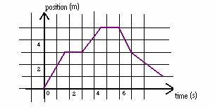
3.1 Consider the following diagram.
a. Discuss the speed in each segment of the graph. Describe in words how you would determine a value for the speed in each segment of the graph.
b. Are you able to determine the direction of motion in each segment in the graph? Could you use a symbol to indicate the direction of motion? Explain. How would you express both the speed and the direction numerically?
Discuss the above with an instructor.
A quantity that expresses both speed and direction is called velocity. The definition of average velocity over a time interval is the displacement during the time interval divided by the time interval. The displacement is the final position minus the initial position and the time interval is the final time minus the initial time. We can write this mathematically as
![]()
or, equivalently, ![]()
xf is the final position and xi is the initial position. tf is the final time and ti is the initial time. The units of velocity are meters per second (m/s). Since displacement is a vector quantity, velocity is also a vector quantity. It has both a magnitude and a direction. The magnitude of the velocity is called the speed.
When working in one dimension, the direction of the velocity can be described as forward or backward, left or right, positive or negative, etc. We will use the words positive or negative or the symbols + or – to describe the direction of the velocity. It is common, when working in one dimension, to write the above equation as a scalar equation, where the average velocity is either a positive or negative quantity depending on the direction of motion
![]() .
.
c. Use the equation for velocity to calculate the average velocity for each segment of the graph. Record your results below.
|
Time
Interval (s) |
Speed
(m/s) |
Direction |
Velocity
(m/s) |
|
0 - 1.5 |
|
|
|
|
1.5 - 3 |
|
|
|
|
3 - 4.5 |
|
|
|
|
4.5 - 6 |
|
|
|
|
6 - 7 |
|
|
|
d. Determine the average velocity over the time interval from 0-4.5s (both the magnitude and the direction). Determine the average velocity over the time interval from 0-7s (both the magnitude and the direction).
Check your calculations with an instructor.
e. Make a graph of velocity vs. time (velocity on the vertical axis and time on the horizontal axis) for the data in part c.
Equipment List:
Motion detector
LabPro Computer Interface
LoggerPro software
4.1
a. Predict and sketch velocity vs. time (time on the horizontal axis, velocity on the vertical axis) graphs for the following situations:
· standing still
· starting near the detector, walking at slow speed away from the detector
· starting away from the detector, walking at a fast speed towards the detector
· standing 3m away from the detector, walking at a slow constant speed towards the detector, stopping briefly, walking at a fast constant speed away from the detector
· walking at a slow constant speed away from the detector, then walking at a fast constant speed further away from the detector
b. Click on this link to the file Position & velocity. The graph of velocity vs. time will be labeled velocity on the y-axis. The motion detector is actually measuring your velocity. Perform the motions described in part a. in front of the motion detector while taking data to test your predictions.
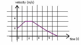
4.2 Consider the following graph of velocity vs. time.
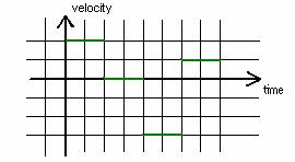
a. Describe in words how you would move
in front of the motion detector in order to
create the graph.
b. Walk in front of the motion detector and try to create the graph.
c. Draw the position vs. time graph that corresponds to the motion of the velocity graph.
Check your graph with an instructor.
4.3 Consider the following position graphs.
a. Calculate the slope of each segment of the graph.
b. Compare the slopes calculated in part a to the average velocity in each of the time segments in part 3.1.c. How do the slopes and the average velocities compare?
c. Discuss the statement: “The velocity is the rate of change of position with time.”
Discuss the statement: “The velocity is the slope of a position vs. time graph.”
4.4
a. What would the velocity vs. time graph look like, if you were to move, not at a constant speed, but getting faster and faster and faster? (This is a prediction. Draw the graph.) What if you were moving slower and slower and slower?
b. If you were to move faster and faster and faster at a constant rate (your velocity is increasing at a constant rate), what would the velocity vs. time graph look like? (This is a prediction. Draw the graph.)
c. Predict the position vs. time graph for part b.
d. Set up the motion detector and test your
predictions to parts a and b.
Equipment List:
Motion detector
LabPro Computer Interface
LoggerPro software
Low Friction Dynamic Track
Cart
Cart with fan accessory
Rod Stand
5.1 Tilt a Dynamics track at a small angle to the table, as in the diagram below.
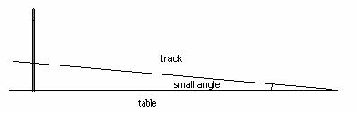
a. Place a cart at the top of the track and release it. Plot the velocity vs. time for the cart, using the motion detector. Is the velocity increasing at a constant rate? Explain how you know.
b. Give a definition of acceleration. It does not have to be formal. (Describe your understanding of what it means to accelerate.)
c. Was the cart in part 5.1.a accelerating? Explain.
The definition of average acceleration over a time interval is the change in velocity during the time interval divided by the time interval. The change in velocity is the final velocity minus the initial velocity and the time interval is the final time minus the initial time. We can write this mathematically as
![]()
or, equivalently, ![]()
where vf is the final velocity and vi is the initial velocity, tf is the final time and ti is the initial time. The units of acceleration are meters per second per second (m/s2). Acceleration is a vector quantity. It has both a magnitude and a direction.
As for velocity, when working in one dimension, the direction of the acceleration can be described as forward or backward, left or right, positive or negative, etc. We will use the words positive or negative or the symbols + or – to describe the direction of the acceleration. It is common, when working in one dimension, to write the above equation as a scalar equation, where the average acceleration is either a positive or negative quantity depending on the direction of motion
![]() .
.
d. Determine the average acceleration of the cart in
part a.
Check your calculation with an instructor.
5.2
a. In each of the four cases below, determine whether the cart is accelerating
- a cart on a flat low friction dynamics track, which has been given an initial push (Determine if it is accelerating after the initial push. )
- a cart on a tilted track, released from the top of the track before it hits the bottom bumper, as in part 5.1.a.
- a cart on a tilted track, as in part 5.1.a, that has been released from the top of the track, allowed to hit the bottom bumper and continue back up the track (consider the motion after it has hit the bumper and is moving up the track)
- a cart with a fan (obtain this from an instructor) on top of it with the fan running, on a flat low friction dynamics track
b. Click on this link to open the file position, velocity, and acceleration and use the motion detector to plot the acceleration vs. time for each of the cases in part 5.2.a. Is the data consistent with your answers to 5.2.a?
c. Consider the following diagram.
(i) Calculate the average acceleration for each segment.
(ii) Calculate the slope of the line for each segment.
d. Discuss the statement: “The acceleration is the rate of change of velocity with time.”
Discuss the statement: “The acceleration is the slope of a velocity vs. time graph.”
e. Use the motion detector to plot position vs. time, velocity vs. time, and acceleration vs. time for a cart on a tilted (at a small angle) low friction dynamics track for a time long enough for the cart to bounce off the bumper three times. Discuss how the acceleration is the slope of the velocity vs. time graph and the velocity is the slope of the position vs. time graph for each segment.
Discuss the graphs with an instructor.
Equipment List:
Motion detector
LabPro Computer Interface
LoggerPro software
Low Friction Dynamic Track
Cart
Rod Stand
Book
Softball
Box
Coffee filter
Aluminum Foil
Super Ball
6.1 Consider the following graph of acceleration vs.
time.
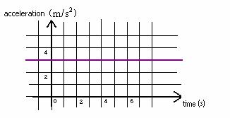
a. For the time interval 2s – 6s, what is the average acceleration? Explain. Would the average acceleration be different for a different time interval? Explain.
b. If the acceleration of an object remains constant, what statement can you make about the average acceleration? Explain.
c. Describe any cases you can think of where the acceleration of a moving object remains constant.
6.2 Hang a motion detector from the ceiling with the side with the sensor towards the floor.
a. Open the position, velocity, and acceleration file and set the experiment length for 1s. Use the motion detector to plot the acceleration vs. time for each of the following cases:
(i) Drop a book from 0.5m below the detector to the floor.
(ii) Drop a softball from 0.5m below the detector to the floor.
(iii) Drop a box from 0.5m below the detector to the floor.
b. Compare the accelerations of the three objects in part 6.2.a. For each object, is the acceleration approximately constant while the object is falling? Explain.
c. Do all objects falling towards the earth fall with the same acceleration? Explain.
d. Use the motion detector to plot the acceleration vs. time for each of the following cases:
(i) Drop a coffee filter from 0.5m below the detector to the floor.
(ii) Drop a piece of aluminum foil from 0.5m below the detector to the floor.
(iii) Drop a super ball from 0.5m below the detector to the floor.
e. For which of the objects you have observed in parts a and d is there very little air friction? For which of the objects you have observed in parts a and d is there a lot of air friction?
Extensive experiments have been done that indicate that all objects fall towards the earth with a constant acceleration if air friction is negligible (there is very little air friction). The magnitude of that acceleration is approximately 9.8m/s2 near the surface of the Earth. The symbol g is often used to represent the magnitude of this acceleration (g = 9.8m/s2).
If you did not get good data for the super ball, look at this file. Take note at the acceleration, on average, it is 9.8m/s2.
f. For the objects you observed in parts a and d for which there was very little air friction, how does the acceleration compare to the value 9.8m/s2?
6.3 Use the motion detector to plot the acceleration vs. time for a cart on a low friction dynamics track tilted at a small angle.
a. While the cart is on the track, except when it hits the bumper, is the acceleration constant? Explain.
b. When the acceleration is constant, describe the graph of velocity vs. time. For the graph in 6.1.a, draw a possible graph of velocity vs. time.
Discuss your answer with an instructor.
c. It can be shown, that for a straight line
graph that the average value between two points on the line is the value of the
point halfway between the two points. For example, for a plot of velocity vs.
time, if the two points chosen are v1 and v2, as shown in
the diagram, below, the average value over the time interval t1 to t2
is ![]() , as shown.
, as shown.
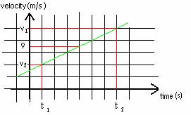
Verify the equation ![]() , using the velocity vs. time graph you generated in 6.3.a.
, using the velocity vs. time graph you generated in 6.3.a.
Since the velocity vs. time graph is always a straight line for the case of constant
acceleration, the equation ![]() is always true for
constant acceleration.
is always true for
constant acceleration.
Equipment List:
Motion detector
LabPro Computer Interface
LoggerPro software
Low Friction Dynamic Track
Cart
Cart with fan accessory
Rod Stand
Meter Stick
7.1 For objects moving at constant acceleration, the three equations below can be applied.
![]()
![]()
![]()
It is also possible to manipulate these three equations to obtain four kinematics equations for use in describing objects moving at constant acceleration. These equations are given below.

where tf – ti, the final time minus the initial time, is the time interval, xf – xi (the final position minus the initial position) is the distance traveled, vi and vf are the initial and final velocities and ā is the acceleration.
These equations are sometimes written as

where t = tf – ti is the time interval.
These equations are valid only for the case of constant acceleration.
a. Set up an experiment with constant acceleration that will allow you to measure position, velocity and acceleration as a function of time with the motion detector and verify the four kinematics equations given above.
b. Have someone hold a meter stick, as the person on the right in the picture below. A second person places his/her hands near the bottom of the meter stick with thumb and forefinger so that they can catch the meter stick when it falls. Record the position of the second person’s thumb and forefinger (what number on the meter stick they are aligned with). Have the person holding the meter stick release the meter stick (The person should just release it all of a sudden.). The second person should catch it as soon as they perceive it is released. Record the position of the person’s thumb and forefinger after they have caught the meter stick. Determine the distance the meter stick fell. Use one of the kinematics equations to determine the person’s reaction time.
Determine the reaction time for each person in your group.

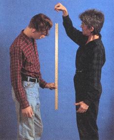
(from Fundamentals of College Physics 2nd Edition by Peter J. Nolan, Wm. C. Brown Publishers, Chicago, 1995)
SUMMARY
You should be able to describe in words the motion of an object that would produce a particular graph of position, velocity or acceleration vs. time. Given the motion of an object, you should be able to draw the position, velocity, and acceleration graphs. Given a particular graph (either position, velocity or acceleration), you should be able to draw other graphs: for example, given a position graph, you should be able to draw the velocity and acceleration graphs. You should understand the mathematical definition of average velocity, be able to use it, and understand that velocity is the rate of change of position and can be found from the slope of the position graph. You should understand the mathematical definition of average acceleration, be able to use it, and understand that acceleration is the rate of change of velocity and can be found from the slope of the velocity graph. You should be able to use the kinematics equations for the case of constant acceleration to describe the motion of moving objects and to solve for unknown parameters.